
Calculation & quality
Once you have entered your survey data, you can have it calculated. CaveRenderPro calculates the 3D coordinates of all survey stations and offers various adjustment methods to improve the accuracy of the survey.
Survey calculation
Starting the calculation
- Make sure that all instruments are defined (File → Properties → Instruments)
- Go to Data → Calculate → Calculate (or
Ctrl+B) - CaveRenderPro calculates the 3D coordinates of all survey stations
- Check for errors: red fields indicate problems
How the calculation works
The coordinates are calculated step by step:
- Origin: the first survey station is calculated from the cave data (latitude, longitude, elevation)
- Survey shots: every further survey station is calculated from the length, azimuth and inclination of the previous survey shot
- Coordinates: the calculated X, Y, Z coordinates are entered into the datasheet
- Views: these coordinates are then used in the visualizations (plan, extended profile, etc.)
LRUD
LRUD means: left, right, up, down – the four cross-section measurements at every survey station.
LRUD types
There are different ways in which LRUD values are calculated:
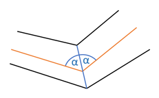
Bisection – the cross-section bisects the angle between the survey shots:
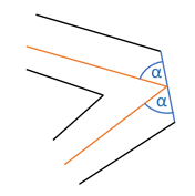
Acute angle – the cross-section follows the more acute angle:
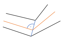
Perpendicular – the cross-section is perpendicular to the survey shot:
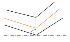
Vertical – vertical cross-sections are shown upright:
Controlling the choice of LRUD types
Under File → Properties → Settings you control which LRUD type is used automatically:
Critical angle vertical (0°–90°) – with a smaller inclination, vertical cross-sections are shown upright:
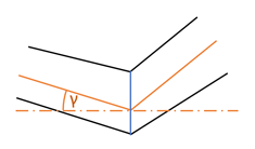
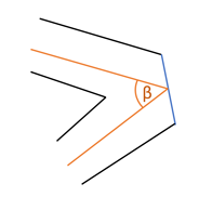
Critical angle acute angle (0°–90°) – with a smaller angle between two lines, cross-sections are shown at the acute angle, otherwise by bisection:
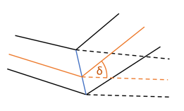
Critical angle junction (0°–90°) – with a smaller angle at junctions, cross-sections are taken over from the branching passage:
LRUD perpendicular – cross-sections are shown perpendicular to the survey shot:
The default values are chosen so that cross-sections and the resulting volumes are depicted well.
A sample file Demo Querschnitt.xml is included.
Manual adjustment
For individual survey stations you can override the LRUD type:
- Open the datasheet (Ctrl+D)
- Click on the LRUD column
- Enter a value (0-3 or -1 to -3)
- Recalculate
| Type | Description | Value |
|---|---|---|
| auto | Determined from the properties | 0 |
| bisection | The cross-section bisects the angle between the survey shots | 1 |
| acute angle | The cross-section follows the more acute angle | 2 |
| perpendicular | The cross-section is always perpendicular to the survey shot | 3 |
| bisection vertical | Like bisection, vertical cross-sections are shown upright | -1 |
| acute angle vertical | Like acute angle, vertical cross-sections are shown upright | -2 |
| perpendicular vertical | Like perpendicular, vertical cross-sections are shown upright | -3 |
Automatic LRUD
CaveRenderPro can calculate LRUD values automatically from splays:
- Select the survey shots and the associated splays
- Go to Data → Calculate → LRUD
- Left, right, up and down are calculated automatically
Selection cone for splays
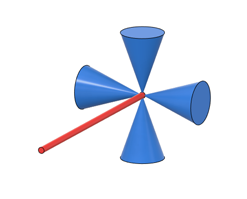
With the angle of the selection cone (File → Properties → Settings) you control which splays are used for an LRUD value:
90° – all splays:
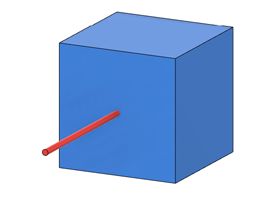
45° – all splays in the corresponding direction (default):
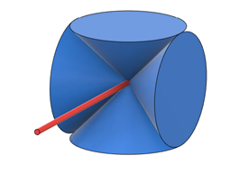
20° – narrow selection cone; if no splay is found, the corresponding value is set to 0:
Direction for the extended profile
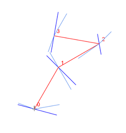
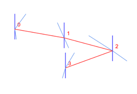
The direction determines how the cross-section measurements (LRUD) are arranged in the extended profile. It controls the arrangement of left and right:
- -1 (left): the left/right measurements are mirrored – left becomes right
- 1 (right): the left/right measurements keep their normal arrangement
A survey traverse with a junction in the plan:
The same traverse unrolled in the extended profile:
Changing the direction
You can set the direction individually for every survey shot:
- Open the datasheet (Ctrl+D)
- Find the Direction column
- Set the value:
-1for left or1for right - Recalculate the data (Ctrl+B)
Calculating the direction
CaveRenderPro can calculate directions automatically from the survey data:
- Go to Data → Calculate → Directions
- The directions are calculated on the basis of the azimuth values
- CaveRenderPro determines automatically whether a survey shot runs to the left or to the right
Visualizing in the layout
You can depict the directions in the visualization as colours:
- Go to Layout → Colours/Textures → Direction
- Survey shots with different directions are shown in different colours
- Splays are coloured according to their own direction
Adjustment and loop closures
Why is adjustment important?
Small errors occur in every survey (measurement errors, calibration, etc.). The adjustment distributes these errors intelligently so that the survey results are consistent.
Under Calculate → Adjustment you find the Analysis, which shows the loop closure errors without an adjustment, and the Adjustment of all loops. Clicking the active button again switches it off.
Analysis of the loop closure errors
Calculate → Adjustment → Analysis
The analysis shows where and by how much the loops fail to close before an adjustment. This way you find measurement errors before they are distributed by the adjustment:
- The survey shots are calculated without an adjustment
- If a survey station gets different positions via different survey shots, these are connected by an error line
- The length of the error line is the error of the loop closure at the survey station
Display of the error lines
- When switching on, Layout → Colours/Textures → Adjustment is selected automatically – the survey shots appear grey
- The error lines are only displayed with the colouring Adjustment
- They are coloured according to the size of the error: the largest error displayed forms the upper end of the scale (red with Rainbow), and the legend shows the corresponding values in metres
Demo Ringschluss.xml and switch on Analysis: the error lines appear at the loop closures, and the statistics list the errors with the largest one at the top.
Adjustment
Calculate → Adjustment → Adjustment (all survey shots in loops)
- Solves an overdetermined system of linear equations so that the squared errors are minimized
- The coordinates of the reference points and the length 0 of the auxiliary points remain fixed
- As far as possible, vertical shafts and chimneys as well as the dive depth are preserved
- The closing error is distributed according to the length of the survey shots: a survey shot 10 m long is adjusted twice as much as one 5 m long
- A weight that has been entered is taken into account in addition
Even large cave systems with several thousand survey shots in loops are adjusted in fractions of a second.
A sample file Demo Ringschluss.xml is included.
Weight values
| Weight | Meaning |
|---|---|
| -1 | Station fixed – the survey shot is adjusted normally, but its end point stays in place |
| 0 | No entry – the survey shot counts normally, like weight 1 (default) |
| 0.5 | Light weighting – the survey shot is changed twice as much (as if surveyed half as accurately) |
| 1 | Normal weighting |
| 2 | Heavy weighting – the survey shot is changed half as much (as if surveyed twice as accurately) |
| 100 | Virtually no adjustment – the survey shot stays practically as it was measured |
A weight acts linearly: weight 2 stands for twice as accurate a survey – the survey shot is changed half as much as a survey shot of the same length with weight 1. Weight 0.5 stands for half as accurate a survey – the survey shot is changed twice as much.
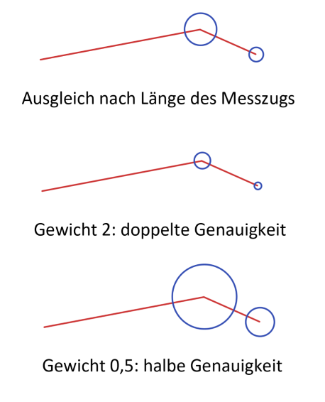
You can set weights in the datasheet in the Weight column. A survey shot that should practically not be adjusted is included with a very large weight (e.g. 1,000,000). A survey station that should stay in place is held with weight -1 on the survey shot leading to that station. If the station is connected to a reference point, the reference point takes precedence.
The weights are taken into account when exporting and importing in the table format and when replacing values (Data → Values with the column Weight).
Adjustment statistics
Calculate → Adjustment → Statistics
The statistics show by how much the adjustment has displaced your survey shots. They can only be switched on when an adjustment or the analysis is active.
For an adjustment there is one row per adjusted survey shot:
| Column | Meaning |
|---|---|
| Survey shot | Passage and station from–to |
| Length | Measured length of the survey shot in metres |
| Weight | Weight entered for the survey shot – with an adjustment |
| Loop (deprecated) | Loop number of the survey shot – only with the loop closure by loop numbers |
| Adjustment | Absolute displacement of the survey shot in metres |
| Error | The same displacement relative, in % of the survey shot length – a short survey shot stands out more here than in the absolute column |
| ΔLength | Change of the length of the survey shot in metres |
| ΔAzimuth, ΔInclination | Change of the direction of the survey shot in degrees. For vertical survey shots (shaft, chimney) ΔAzimuth stays 0, because no direction is defined there |
| ΔX, ΔY, ΔZ | Displacement in each direction |
| The six Δ columns show the change with its sign, but sorting is by magnitude – so the largest changes are at the top, no matter in which direction they go. | |
Which survey shots appear depends on the type of adjustment: with the Adjustment all survey shots in a loop, with the loop closure by loop numbers all those that actually lie in the loop.
Statistics with the analysis
With the Analysis there is one row per loop closure error:
| Column | Meaning |
|---|---|
| Cave | Cave of the survey station |
| Survey Station | Passage and station of the survey station with different positions |
| Error | Distance between the two positions in metres – the length of the error line |
| ΔX, ΔY, ΔZ | Distance in each direction in metres, with its sign |
The table is pre-sorted by Error in descending order. The statistics list all errors of the selected caves, regardless of which survey shots are selected in the visualization. Clicking on a row selects the survey shot that leads to the deviating position.
Sorting and looking up
The table is pre-sorted by Error (%) in descending order, with the station adjustment by Adjustment (m): the largest displacements are at the top – the best candidates for a measurement error. All eight numeric columns can be sorted in descending order by clicking the heading; a second click undoes the sorting and restores the order of the datasheet.
Station adjustment (deprecated)
With File → Properties → Settings → Station adjustment the adjustment is done without taking the length into account, as it was up to release 26.8.2:
- The closing error is distributed evenly over all survey shots – a short survey shot is changed just as much as a long one
- A weight acts quadratically: a survey shot with weight 2 is changed only a quarter as much as one with weight 1
- The statistics are sorted by Adjustment (m), and the colouring Adjustment shows the displacement in metres
The setting is stored in the file.
Loop closure by loop numbers (deprecated)
The loop closure by loop numbers is no longer recommended and is hidden in the ribbon by default. You can show it again under File → Properties → Settings → Show loop closure; the setting is stored in the file. As long as it is hidden, caves that were saved with Loop are calculated with Adjustment when they are opened.
Calculate → Adjustment → Loop
Loops are closed one after the other by linear interpolation:
- Give all survey shots of a loop that are to be adjusted the same loop number
- Carry out the loop closure
The loops are closed in ascending order (e.g. 1, 3, 4, 6).
Visualizing the adjustment
You can see the adjustment in the visualization:
- When the adjustment is switched on, Layout → Colours/Textures → Adjustment is selected automatically
- Every survey shot is coloured according to its error in %, with the station adjustment according to the adjustment in metres – the same value as in the adjustment statistics
- Splays get the colour of the survey shot they are attached to
- Grey: no adjustment
- Violet: small adjustment
- Red: largest adjustment in the plan
The scale is relative: the survey shot displaced the most always forms the upper end, and all others are measured against it. The legend (Visualization → Legend) shows the corresponding values in %, with the station adjustment in metres.
With the Analysis the survey shots are grey, and the error lines are coloured according to the size of the error. The legend then shows the errors in metres, with 0.00 m grey as with the adjustment.
Data reduction
The group Calculate → Data Reduction shows the key figures of the selected caves:
| Value | Meaning |
|---|---|
| Survey Shots | Number of survey shots |
| Splays | Number of splays |
| Adjustment | Number of adjusted survey shots |
| Total Length | Total length of the survey shots in metres |
| Total Depth | Total depth in metres |
| Extension | Horizontal extension in metres |
| Highest Station / Lowest Station | Highest and lowest survey station in metres |
These values can also be inserted into drawing texts as variables – see Drawings & plans → text with variables. How the horizontal extension is calculated is described in the chapter Mathematics.
North alignment
In the group Calculate → North you define what the depiction is aligned to:
- Geographic – alignment to geographic north
- UTM Grid – alignment to grid north; the meridian convergence is calculated for every entrance
For drawings spanning several caves, UTM Grid has to be selected. For the calculation of the meridian convergence see Mathematics.
Connecting caves
Several caves in one system
You can connect several caves with each other if they are physically connected:
Steps:
For connections between caves, the coordinates of cave entrances or of connections can be used as the connecting point.
- Create a reference point (RefStation = Station)
- Enter the cave number of the other cave in the column RefCave (double-click)
- Recalculate – the coordinates are taken over automatically
Connection variants
Variant 1: attaching to a cave entrance
- One cave is attached to the entrance of the other
- The reference point takes on the coordinates of the entrance
- Quick and simple
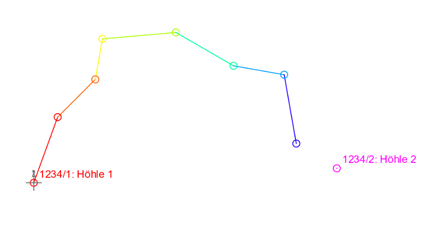
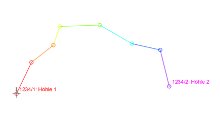
Variant 2: attaching two reference points to one connection
- One reference point is defined in each of the two caves
- Both are attached to the same connection
- More flexible when the connection is not at the entrance
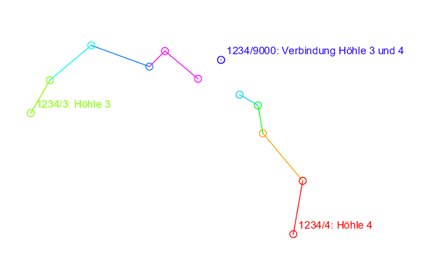
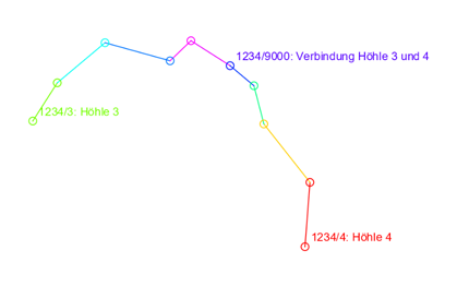
A sample file Demo Verbindung.xml is included.
Tips for better results
- Instrument calibration: calibrate your survey instruments regularly
- Careful recording: note all measured values precisely in the field or use digital instruments
- Repeated measurements: measure critical places several times
- Compass: keep metal parts and electronic devices away from your compass - they distort the measurement considerably
- Reference points: set reference points by surface surveys
- Across caves: connect neighbouring caves to improve the overall accuracy
Next steps
Now your data is calculated and checked. The next step:
- Visualization - see your survey data as a graphic