
Visualization
Once your survey data is calculated, you can visualize it! CaveRenderPro offers many different types of depiction: from classic plans through 3D perspective to interactive maps.
Opening the Visualization tab
Click on the tab Visualization (or press Ctrl+G) to start the visualization.
Here you see:
- Selection of the view type (top) – choose a view
- Visualization area (centre) – the current view
- Status bar (bottom) – information about the current view
View types
| Name | Shortcut | Explanation |
|---|---|---|
| Plan (top view) | Ctrl+1 |
Overall overview of the cave. |
| Extended profile (side view) | Ctrl+2 |
Section along the survey shots. The direction and length of the survey shots is defined by the value Direction (e.g. left=-1, right=1). |
| Projected profile (cross-section) | Ctrl+3 |
Vertical section through the cave. |
| Perspective (3D view) | Ctrl+4 |
Survey shots in perspective. With Orthogonal you switch to the orthogonal projection. |
| Volumes (3D hull) | Ctrl+5 |
3D volume view as a hull built from the splays; survey shots without enough splays use the calculated LRUD values. |
| Map | Ctrl+6 |
Show survey shots on a map. With Map selection you choose the map, with UTM Grid you show the grid. |
Operation with mouse and keyboard
2D views (plan, extended profile, projected profile)
| Action | Mouse | Keyboard |
|---|---|---|
| Zoom | Mouse wheel: scroll up/down | Ctrl+↑ / Ctrl+↓ |
| Pan | Right-click + move | Shift + arrow keys |
| Overview | - | Ctrl+Shift+Z = show everything |
3D views (perspective, volumes)
| Action | Mouse | Keyboard |
|---|---|---|
| Zoom | Mouse wheel: scroll up/down | Ctrl+↑ / Ctrl+↓ |
| Zoom (slowly) | Mouse wheel: Ctrl + scroll up/down |
- |
| Rotate | Left-click + move | Arrow keys |
| Pitch | Left-click + move + release | - |
| Pan | Right-click + move | Shift + arrow keys |
| Overview | - | Ctrl+Shift+Z = show everything |
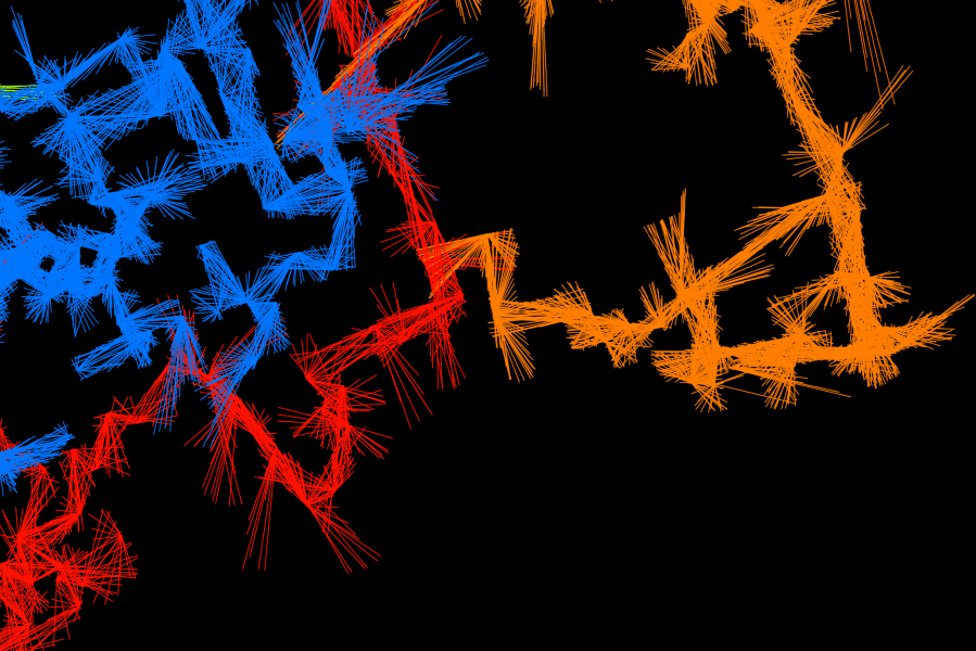
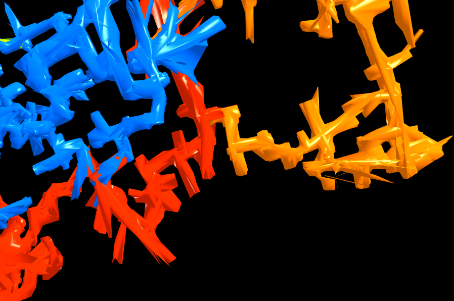
Volumes: 3D hull from splays
The volume view and the 3D model export (Visualization → Visualization → 3D Model) use a hull model that reconstructs the shape of the passage from the splays:
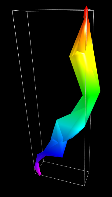
For every survey station, its own splays determine how the wall is depicted there:
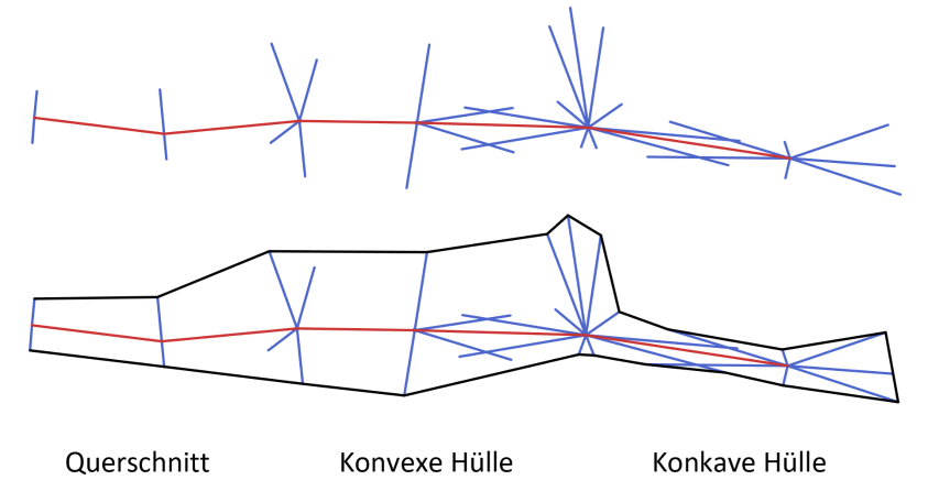
- Fewer than 3 splays: the station only contributes its LRUD values. If both stations of a survey shot have too few, the classic tube is created from the LRUD values or from the default LRUD values in the properties
- Convex hull: the normal case with at least 3 splays. Unsurveyed space remains between the two stations, and a convex hull bridges it across the whole survey shot
- Concave hull: if the splays of one station and those of its neighbour overlap along the survey shot by at least half its length, the passage in between is surveyed completely. Instead of the bridge, the station then gets a concave hull built only from its own splays — recesses and niches are preserved, and unsurveyed areas close up towards the station. If a convex hull meets such a station, only the splays measured across the survey shot support it there — otherwise it would cover up its niches again
- A very large number of splays around a station is thinned out on a 4° grid: per direction the shortest splay counts (the nearest wall). At concave stations the full point density is preserved
- Consecutive survey shots share the splays of the station they have in common — neighbouring hulls therefore merge seamlessly
- Individual stations (survey shots of length 0) get a hull built from their own splays
With right mouse button → survey shot you can examine the hull of a single survey shot.
- Clicking on a station or a splay selects the survey shot with all of its splays
- A click that hits nothing switches the filter off; the selection of the records is preserved
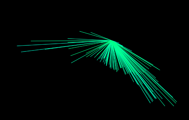
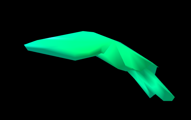
To optimize the hull, individual disturbing survey or auxiliary points can be switched off directly in the 2D or 3D plan via the context menu (right mouse button → Deactivate). They are switched back on via the datasheet (right mouse button → de-/reactivate).
How a station is treated can be prescribed in the datasheet in the field Hull: 0 auto, 1 LRUD, 2 convex hull or 3 concave hull. The value belongs to the station in that row and therefore applies to all survey shots that end or start there. If a station has fewer than 3 splays, the LRUD values are used even with a fixed setting. The field is stored in the cave file.
Tips for surveying
To make the hull look good in the cave, it helps to set survey stations and splays following a few simple rules:
Survey stations
- One station at every junction — and a survey traverse of its own into every branch. A station always surveys only one passage.
- An additional station when one station cannot see the shape — behind a sharp bend or in a large chamber.
- Use every station name only once.
Splays
- Measure all around — left, right, up, down and diagonally in between. Not only to one side.
- Always aim at the nearest wall, as straight on as possible. The length is the distance to the wall.
- Only measure real walls — not into empty space, not into niches, not at stalactites.
- No outliers — keep all splays of a station similar in length, no single long shot.
- Do not measure forwards or backwards along the passage.
- Stay in your own passage — never measure into a neighbouring passage.
- At least 3, better 6–8 splays per station, the same number everywhere.
2D areas from splays
As the two-dimensional counterpart to the 3D hull, the area of the passage can be depicted from the splays with Layout → Survey Shots → Areas — in the 2D plans (plan, extended profile, projected profile) and in the map views:
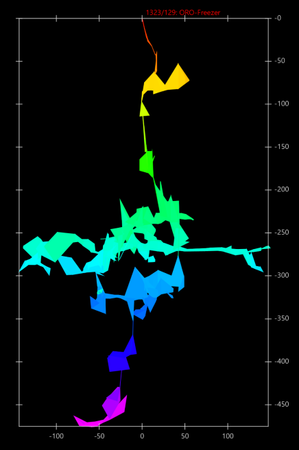
- The same rules apply as for the 3D hull: densely surveyed stations get a concave outline from their own splays, otherwise a convex area is created across the survey shot — in the plan and in the maps in the plan plane, in the extended profile and in the projected profile in the respective section plane
- The classification is calculated once for all views: a station is therefore not treated differently in the plan than in the projected profile or in the 3D view
- Consecutive survey shots share a station and overlap there, so that the passage is filled without gaps
- Individual stations without a connected survey shot get an area from their own splays, as in the 3D model
- Stations with fewer than 3 splays still use the LRUD values
- With an active filter the areas are calculated as in the complete plan, and the filter only shows a part of it (for the export to KML and GeoJSON only the filtered survey shots are taken into account)
- The areas are also taken into account in the export to Google Earth (KML) and GeoJSON
Map views
CaveRenderPro shows your cave on base maps to give it a geographic context. You choose the map in the ribbon with Map selection. The following maps are included:
| Map | Description | Zoom | Source |
|---|---|---|---|
| OpenTopoMap | Topographic map worldwide with contour lines | 17 | OpenTopoMap / OpenStreetMap |
| OnlineTopoMap | Topographic map worldwide in HD resolution. For the display without a watermark, request an API key at onlinetopomap.com and enter it under File → Properties → Settings | 18 | Top-O-Map / OpenStreetMap |
| CyclOSM | Cycling and hiking routes worldwide | 19 | CyclOSM / OpenStreetMap |
| Thunderforest | Landscape map with relief. For the display without a watermark, request a free API key at thunderforest.com and enter it under File → Properties → Settings | 19 | Thunderforest |
| WorldImagery | Satellite images worldwide. How up to date they are varies by region | 19 | Esri |
| basemap.at | Official map of Austria | 19 | basemap.at |
| swisstopo | National map of Switzerland in HD resolution | 18 | swisstopo |
| Plan IGN | Official map of France | 19 | IGN |
| Google Earth | External application. Export your cave as a KML file and open it in Google Earth for a 3D visualization. | – | Google Earth |
Under File → Properties → Maps you define which maps appear in the map selection, and you can add your own maps – see Settings → Maps.
Notes on the map cache
CaveRenderPro stores downloaded map data locally in order to improve performance and save bandwidth:
- Automatic caching: map tiles are stored automatically the first time you load them
- Offline use: map sections that are already cached can be used offline
- Cache storage: the cache is located in the subfolder
cachenext to the cave file, with a separate subdirectory per map named after the map (e.g.cache/OpenTopoMap; with an API keycache/ThunderforestKeyorcache/OnlineTopoMapKey), and it takes up disk space - Clearing the cache: File → Tools → Clear cache removes the subfolder
cacheof all recently opened files after a confirmation. You delete the cache of a single map under File → Properties → Maps with Clear cache
Drawings on the map
In the tab Drawings the drawings of the plan can also be selected for the map, and they are displayed on top of the map. With the button Map or with Ctrl+6 you switch there between plan, extended profile, projected profile and map without leaving the tab. Drawing itself still happens in the plan, which is why the tab Elements switches there. The map has its own selection: the first time it is taken over from the plan, after that both views stay independent.
As long as a drawing is displayed, no survey shots appear on top of the map — the drawing takes their place. In the tab Visualization the map shows the survey shots as before. With Calculate → North → UTM Grid the drawing is rotated by the meridian convergence, because the map is always oriented to true north.
Selecting survey shots
Selection filter
With Layout → Survey Shots → Filter you display only certain survey shots:
| Filter option | Description |
|---|---|
| Level | Filters by level numbers |
| Passage | Filters by passage numbers |
| Year | Filters by the year of the survey (YYYY) |
| Month | Filters by the month of the survey (YYYYMM) |
| Day | Filters by the day of the survey (YYYYMMDD) |
| Depth | Filters by the depth of the survey shots |
| Height | Filters by the height of the survey shots |
| Sea Level | Filters by the absolute height above sea level |
| ID | Filters by the ID of the survey shots |
| Selection | Shows only the selected survey shots |
Syntax of the filter selection
With all filters except Selection you can use the following syntax:
- Single values:
25— shows only survey shots with exactly the value 25 - Range:
1-5— shows survey shots in the range from 1 to 5 (inclusive) - Several ranges:
1-5, 10-20, 25— combines several filters with a comma - From ... to the end:
100-— shows all survey shots from value 100 upwards - From the beginning to ...:
-50— shows all survey shots from the beginning up to value 50
Graphical selection
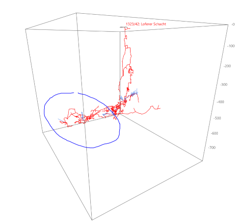
In the line views you can select survey shots graphically, directly with the mouse, by rectangle, lasso or polygon. The modifier key determines the shape, the mouse button the effect:
| Shape | Add | Remove |
|---|---|---|
| Rectangle | Ctrl + left mouse button |
Ctrl + right mouse button |
| Lasso | Alt + left mouse button |
Alt + right mouse button |
| Polygon | Ctrl+Alt + left mouse button |
Ctrl+Alt + right mouse button |
The mouse pointer shows the shape (a square for the rectangle, a lasso or a pentagon for the polygon) and the effect: + for adding, - for removing. The shape being drawn is shown in red.
Rectangle selection (Ctrl)
- Drag a rectangle over the survey shots with the mouse button held down
- On release, all enclosed survey shots are taken over
Lasso selection (Alt)
- Drag along the mouse path with the mouse button held down to enclose survey shots
- On release, all enclosed survey shots are taken over
Polygon selection (Ctrl+Alt)
- Set corner points with the mouse button held down (dragging = line segment)
- A click without moving completes the polygon
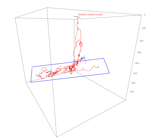
Selecting single stations
A click without moving on a survey station acts directly on that station – with Ctrl or Alt:
- Left mouse button: select the station
- Right mouse button: remove the station from the selection
Layout and display options
The tab Layout offers options for adapting the visualization:
Background
Three backgrounds for the volume and line views (Visualization tab): white, gray and black.
- White: white background (default)
- Gray: gray gradient as the background
- Black: black background for better contrast
Design
Border and north arrow, title information and general display options of the view:
- Border: shows a mapping border around the view
- Gridlines: shows a coordinate grid
- North: shows the direction of north
- Cave Title: display the name of the current cave
- File Name: display the name of the project file
- Worksheet: display the name of the current worksheet
- Orthogonal: show lines and volumes in orthogonal projection instead of in perspective
- UTM Grid: show the UTM grid on the map
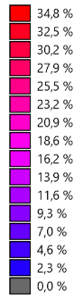
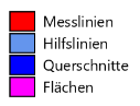
- Legend: show or hide the colour legend at the left edge (for the content per colour mode see below)
Content of the legend per colour mode
The content of the legend depends on the colour that is set (under Layout → Colours/Textures):
| Colour | The legend shows |
|---|---|
| Default | Survey shots, splays, LRUD, areas |
| By depth | Colour scale with height/depth values (follows the height reference entrance or sea level) |
| By date | The date values that occur – per colour the first (earliest) value |
| By adjustment | Scale in metres (0 m = grey); with the analysis, the errors of the error lines in metres |
| By line / level / cave / surveyor | Only the colours in use, with labels (if there are several matches per colour, they are listed) |
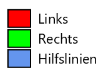
| By direction | Left, right |
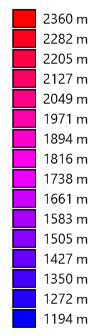
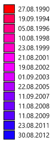
Survey stations
Marking of the survey stations as well as LRUD and cross-sections. Of the buttons Line, Circle and LRUD, only one is active at a time:
- Line: show survey stations marked by a line
- Circle: show survey stations marked by a circle
- LRUD: show LRUD
- Cross-Sections: show cross-sections
Labels
- Cave: display cave names
- Station: display passage/station number
- Title: display station titles
- Depth: display depth or height above sea level of the station
- Info: display information
- Material: display material
- Tasks: display tasks
Survey shots
- Splays: show splays
- Cuboids: show LRUD cuboids
- Areas: areas for 2D plans and maps
Colours
Choose a colour coding for your survey shots:
| Colour coding | Description |
|---|---|
| Default | Default colour for all survey shots (can be changed in File → Properties → Colours) |
| Lines | Colour by line colour (can be changed in File → Properties → Colours) |
| Depth | Colour coding by the height of the survey shot (with a selectable gradient) |
| Date | Colour by the day of the survey (with a selectable gradient) |
| Adjustment | Shows the extent of the adjustment (with a selectable gradient, grey = 0); with the analysis also the error lines, coloured by the size of the error |
| Direction | Colour by the direction of the survey shot (left = red, right = green); splays by their own direction |
| Level | Different colours per level |
| Surveyor | Different colours per surveyor |
| Cave | Different colours per cave |
Selectable gradients
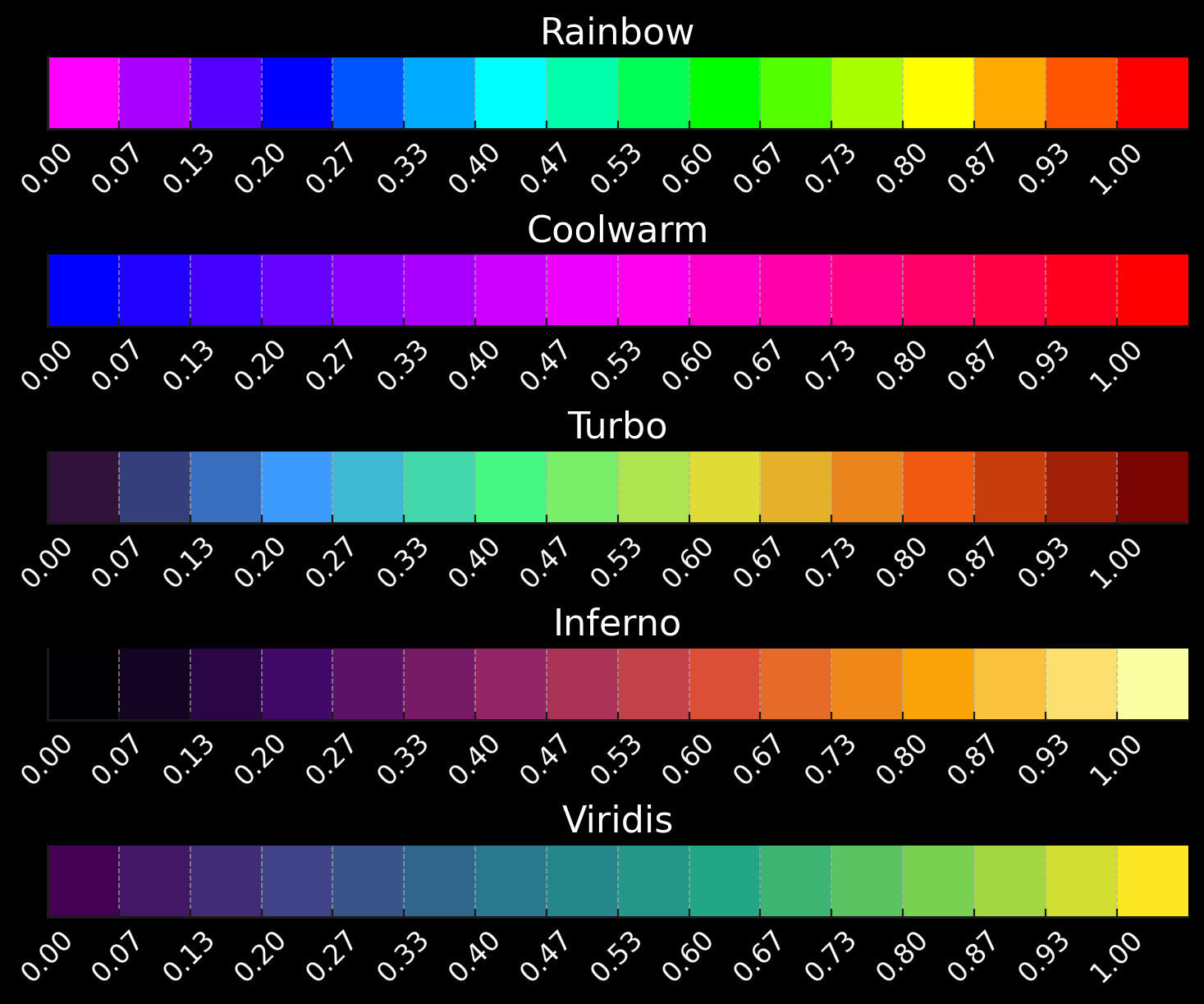
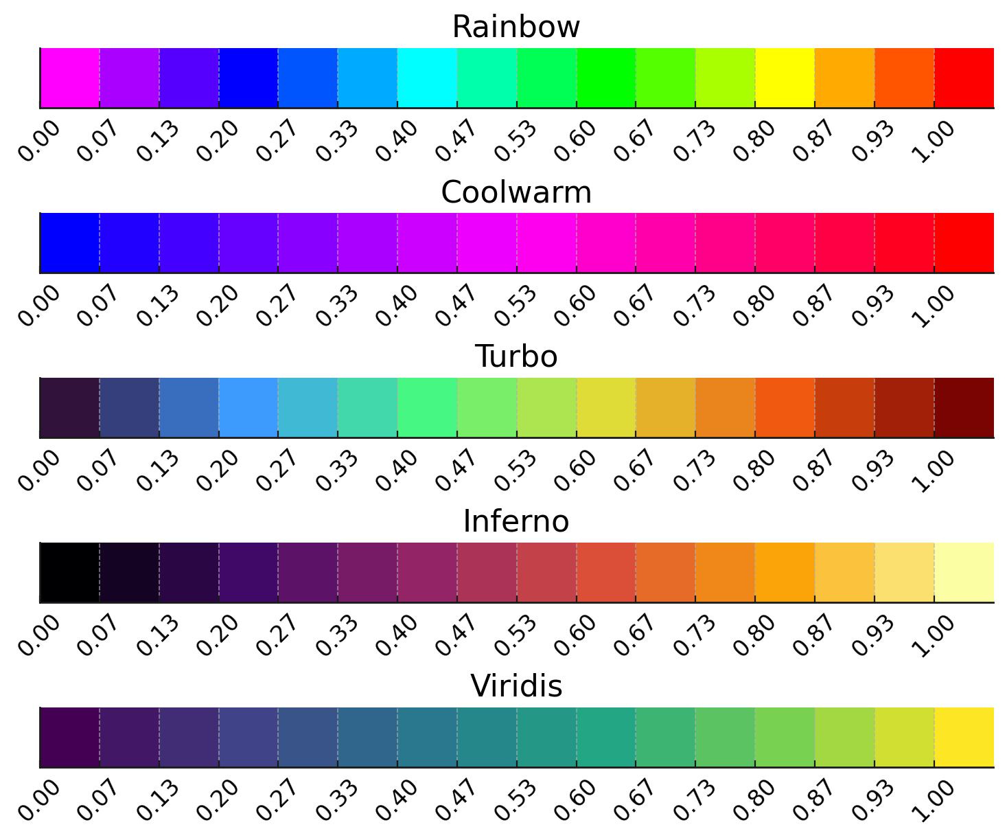
With the colouring by depth, date or adjustment you can choose between 5 different gradients:
| Gradient | Characteristic | Best used for | Special feature |
|---|---|---|---|
| Rainbow | Spectral red-yellow-green-blue-violet | Classic depiction of height | Evenly distributed across the spectrum |
| Coolwarm | Blue → magenta → red | Harmonious, intuitive depiction | Soft transition without harsh jumps |
| Turbo | Finely graded modern spectral map | Detailed differences in depth | High resolution, many intermediate steps |
| Inferno | Black → orange → yellow | High dynamics, dramatic effects | Glowing gradient, very high contrast |
| Viridis | Blue-green → green → yellow | Scientific visualization | Balanced and colour-blind friendly |
How to set the gradient
- Go to File → Properties → Colours
- Choose one of the 5 available gradients
- Then go to Layout → Colours/Textures and choose "Depth", "Date" or "Adjustment"
- The new gradient is applied immediately
Contour lines
- Load: load contour lines from a file
- Display: display loaded contour lines (in the perspective)
Animation
In the group Visualization → Animation you create a camera flight through the cave with any number of positions.
Defining camera positions
- Set up the view you want in 3D (perspective or volumes)
- Save (
Ctrl+Shift+S) stores the current position - Repeat this for further positions
| Function | Description | Shortcut |
|---|---|---|
| Play | Start and stop the animation | Space |
| 360° | Create a 360° animation | – |
| New | Delete all positions | – |
| Start | Jump to the start position | Ctrl+Shift+Home |
| Previous / Next | Previous or next position | Ctrl+Shift+← / → |
| Save | Save the current position | Ctrl+Shift+S |
| Insert | Insert a position | Ctrl+Shift+E |
| Delete | Remove a position | – |
When switching between the positions, the current position is shown in the status bar. You set the animation time in seconds under File → Properties → Settings.
Tips for the best results
- Several views: use worksheets to store different views
- Configuring colours: the right colour coding makes differences visible
- Adjusting the zoom: use the zoom to see details or to get an overview
- 3D perspective: change the viewing direction to understand spatial structures
- Creating an animation: a good animation explains geometry better than static images
Frequently asked questions
Q: The cave is not visible on the map!
A: Check whether you have entered coordinates (latitude/longitude) in the cave data. Without coordinates the map cannot georeference the cave.
Q: Why is the 3D view so slow?
A: The volume view can be slow with a large number of survey shots. Try the perspective view instead, or reduce the number of survey shots (filter).
Q: How do I save a nice view?
A: Use worksheets! Set up your visualization and go to Caves → Worksheets → Update. The setting is saved.
Q: Can I use the map offline?
A: The map views need an internet connection. But once the maps have been loaded, they are loaded from the cache directory. With File → Tools → Clear cache you can remove these directories again.
Next steps
The visualization is the heart of the cave analysis. The following chapters show you how to build on it:
- Drawings & plans - create professional cave plans